Concatenating a gridded rainfall reanalysis dataset into a time series#
General Preprocessing Standard Python
![]()
![]()
![]()
![]()
![]()
Context#
Purpose#
To load and extract a region of interest from a gridded rainfall reanalysis dataset, and concatenate into a time series using the Iris package.
Preprocessing description#
Time series data allows us to carry out a wide range of analyses including but not limited to trend, seasonality, anomaly detection and causality. As most of the climatological datasets are gridded, we provide a general tool to preprocess them into time series. The example global dataset from NCEP/NCAR reanalysis has a fairly low resolution (T62 Gaussian grid or approximately 1.9 * 1.9 degrees lat/long) which allows easy execution. It is openly available with a variety of atmospheric variables at near surface levels in daily and monthly frequencies as well as long-term monthly mean in NetCDF format, which is described in and can be obtained from the NOAA Physical Sciences Laboratory.
This notebook uses a single sample data file for global daily precipitation rate (monthly mean) included with the notebook.
Highlights#
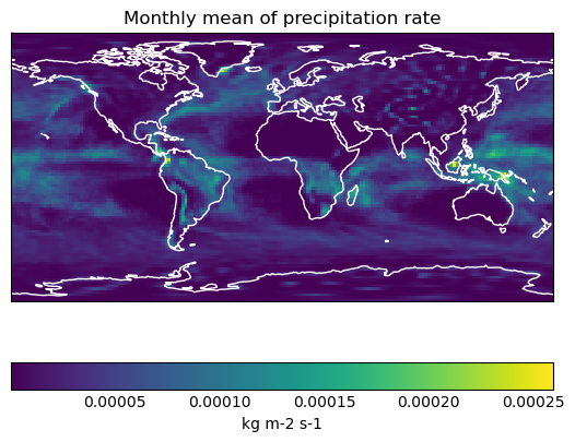
Data for the entire globe is loaded and plotted using Iris
Seasonal means are created by aggregating the data
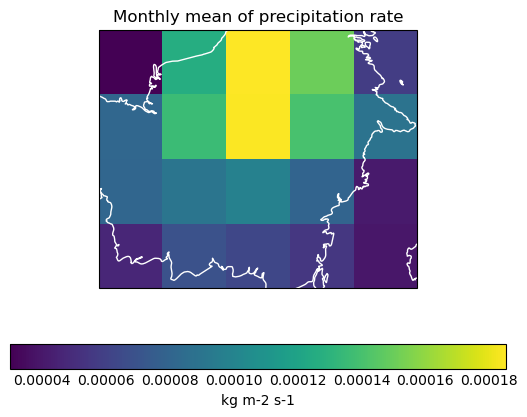
The Indonesian Borneo region is extracted and plotted
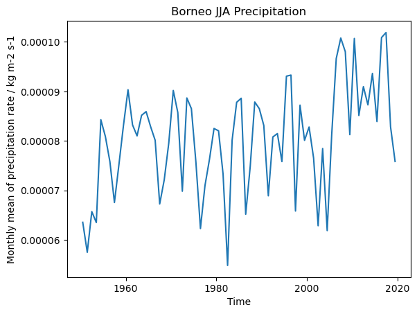
The area-averaged time series for Indonesian Borneo region is created
A particular season and timeframe are extracted from the time series
Contributions#
Notebook#
Timothy Lam (author), University of Exeter, @timo0thy
Marlene Kretschmer (author), University of Reading, @MarleneKretschmer
Samantha Adams (author), Met Office Informatics Lab, @svadams
Rachel Prudden (author), Met Office Informatics Lab, @RPrudden
Elena Saggioro (author), University of Reading, @ESaggioro
Nick Homer (reviewer), University of Edinburgh, @NHomer
Alejandro Coca-Castro (reviewer), The Alan Turing Institute, @acocac
Dataset originator/creator#
NOAA National Center for Environmental Prediction (creator)
Dataset documentation#
E. Kalnay, M. Kanamitsu, R. Kistler, W. Collins, D. Deaven, L. Gandin, M. Iredell, S. Saha, G. White, J. Woollen, Y. Zhu, M. Chelliah, W. Ebisuzaki, W. Higgins, J. Janowiak, K. C. Mo, C. Ropelewski, J. Wang, A. Leetmaa, R. Reynolds, Roy Jenne, and Dennis Joseph. The ncep/ncar 40-year reanalysis project. Bulletin of the American Meteorological Society, 77(3):437 – 472, 1996. URL: https://journals.ametsoc.org/view/journals/bams/77/3/1520-0477_1996_077_0437_tnyrp_2_0_co_2.xml, doi:10.1175/1520-0477(1996)077<0437:TNYRP>2.0.CO;2.
Pipeline documentation#
Marlene Kretschmer, Samantha V. Adams, Alberto Arribas, Rachel Prudden, Niall Robinson, Elena Saggioro, and Theodore G. Shepherd. Quantifying causal pathways of teleconnections. Bulletin of the American Meteorological Society, 102(12):E2247 – E2263, 2021. URL: https://journals.ametsoc.org/view/journals/bams/102/12/BAMS-D-20-0117.1.xml, doi:10.1175/BAMS-D-20-0117.1.
Note
NCEP-NCAR Reanalysis 1 data provided by the NOAA PSL, Boulder, Colorado, USA, from their website at https://psl.noaa.gov
Load libraries#
Show code cell source
import os
import iris
import iris.quickplot as qplt
import iris.coord_categorisation as coord_cat

import cf_units
import nc_time_axis

import matplotlib.pyplot as plt

import urllib.request

import holoviews as hv
import geoviews as gv

import warnings
warnings.filterwarnings(action='ignore')

%matplotlib inline
hv.extension('bokeh')


Set project structure#
notebook_folder = './notebook'
if not os.path.exists(notebook_folder):
    os.makedirs(notebook_folder)
Retrieve and/or load a sample data file#
filepath = 'https://downloads.psl.noaa.gov/Datasets/ncep.reanalysis.derived/surface_gauss/'
filename = 'prate.sfc.mon.mean.nc'

if not os.path.exists(os.path.join(notebook_folder,filename)):
    urllib.request.urlretrieve(os.path.join(filepath,filename), os.path.join(notebook_folder, filename))
# Load monthly precipitation data into an iris cube
precip = iris.load_cube(os.path.join(notebook_folder, filename), 'Monthly Mean of Precipitation Rate')
precip.coord('latitude').guess_bounds()
precip.coord('longitude').guess_bounds()
print(precip)
Monthly Mean of Precipitation Rate / (unknown) (time: 914; latitude: 94; longitude: 192)
    Dimension coordinates:
        time                                        x              -              -
        latitude                                    -              x              -
        longitude                                   -              -              x
    Attributes:
        Conventions                            'COARDS'
        NCO                                    '20121013'
        References                             'http://www.psl.noaa.gov/data/gridded/data.ncep.reanalysis.derived.htm...
        actual_range                           array([-2.3283064e-10, 5.8903999e-04], dtype=float32)
        dataset                                'NCEP Reanalysis Derived Products'
        dataset_title                          'NCEP-NCAR Reanalysis 1'
        description                            'Data is from NMC initialized reanalysis\n(4x/day).  It consists of T42...
        history                                'Mon Jul  5 23:55:54 1999: ncrcat prate.mon.mean.nc /Datasets/ncep.reanalysis.derived/surface_gauss/prate.mon.mean.nc...
        invalid_units                          'Kg/m^2/s'
        least_significant_digit                0
        level_desc                             'Surface'
        parent_stat                            'Individual Obs'
        platform                               'Model'
        precision                              1
        statistic                              'Mean'
        title                                  'monthly mean prate.sfc from the NCEP Reanalysis'
        valid_range                            array([-400., 700.], dtype=float32)
        var_desc                               'Precipitation Rate'
From print(precip) we have an idea whether the metadata is complete and where the possible gaps are. In case the iris cube does not contain a unit, we can set it as follows:
# Set unit of precipitation data, if the cube does not contain it
unit_to_add = 'kg m-2 s-1'
if precip.units == 'unknown':
    precip.units = cf_units.Unit (unit_to_add)
Visualisation#
Here we use the Iris quickplot wrapper to matplotlib (static plot with limited interactivity), and holoviews to interactive plotting the gridded data with added coastline.
Static plot#
Show code cell source
# Plot data of the first time step using iris quickplot with pcolormesh
qplt.pcolormesh(precip[0])
plt.gca().coastlines(color='white')
plt.show()
Interactive plot#
Show code cell source
# Declare some options
options = dict(width=600, height=350, yaxis='left', colorbar=True,
               toolbar='above', cmap='viridis', infer_projection=True, tools=['hover'])

# Create a geoviews dataset object
rainfall_ds = gv.Dataset(precip[0], ['longitude', 'latitude'], 'Monthly Mean Of Precipitation Rate (kg m-2 s-1)',
                             group='Monthly mean of precipitation rate')

plot_rainfall = rainfall_ds.to.image().opts(**options) * gv.feature.coastline().opts(line_color='white')
plot_rainfall
WARNING:param.Image01635: Image dimension latitude is not evenly sampled to relative tolerance of 0.001. Please use the QuadMesh element for irregularly sampled data or set a higher tolerance on hv.config.image_rtol or the rtol parameter in the Image constructor.
Create seasonal means#
Here we construct seasonal means from the monthly data for each grid, for the purpose of extracting a particular season of interest later on.
# Add auxiliary coordinates to the cube to indicate each season
coord_cat.add_season(precip, 'time', name='clim_season')
coord_cat.add_season_year(precip, 'time', name='season_year')
print(precip)
Monthly Mean of Precipitation Rate / (kg m-2 s-1) (time: 914; latitude: 94; longitude: 192)
    Dimension coordinates:
        time                                           x              -              -
        latitude                                       -              x              -
        longitude                                      -              -              x
    Auxiliary coordinates:
        clim_season                                    x              -              -
        season_year                                    x              -              -
    Attributes:
        Conventions                               'COARDS'
        NCO                                       '20121013'
        References                                'http://www.psl.noaa.gov/data/gridded/data.ncep.reanalysis.derived.htm...
        actual_range                              array([-2.3283064e-10, 5.8903999e-04], dtype=float32)
        dataset                                   'NCEP Reanalysis Derived Products'
        dataset_title                             'NCEP-NCAR Reanalysis 1'
        description                               'Data is from NMC initialized reanalysis\n(4x/day).  It consists of T42...
        history                                   'Mon Jul  5 23:55:54 1999: ncrcat prate.mon.mean.nc /Datasets/ncep.reanalysis.derived/surface_gauss/prate.mon.mean.nc...
        invalid_units                             'Kg/m^2/s'
        least_significant_digit                   0
        level_desc                                'Surface'
        parent_stat                               'Individual Obs'
        platform                                  'Model'
        precision                                 1
        statistic                                 'Mean'
        title                                     'monthly mean prate.sfc from the NCEP Reanalysis'
        valid_range                               array([-400., 700.], dtype=float32)
        var_desc                                  'Precipitation Rate'
# Aggregate by season
annual_seasonal_mean = precip.aggregated_by(
    ['clim_season', 'season_year'],
    iris.analysis.MEAN)
# Check this worked
for season, year in zip(
    annual_seasonal_mean.coord('clim_season')[:10].points,
    annual_seasonal_mean.coord('season_year')[:10].points):
    print(season + ' ' + str(year))
djf 1948
mam 1948
jja 1948
son 1948
djf 1949
mam 1949
jja 1949
son 1949
djf 1950
mam 1950
Extract Borneo region#
Here we extract our area of study which covers the Indonesian Borneo region, as specified by Melendy et al. (2014) (available at https://daac.ornl.gov/CMS/guides/CMS_LiDAR_Indonesia.html).
# Create a constraint for the latitude and Longitude extents
Borneo_lat = iris.Constraint(latitude=lambda v: v > -4.757 and v <= 3.211 )
Borneo_lon = iris.Constraint(longitude=lambda v: v > 107.815 and v <= 117.987 )

# Extract data based on the spatial extent
Borneo =  annual_seasonal_mean.extract(Borneo_lat & Borneo_lon)
print(Borneo)
Monthly Mean of Precipitation Rate / (kg m-2 s-1) (time: 305; latitude: 4; longitude: 5)
    Dimension coordinates:
        time                                           x              -             -
        latitude                                       -              x             -
        longitude                                      -              -             x
    Auxiliary coordinates:
        clim_season                                    x              -             -
        season_year                                    x              -             -
    Cell methods:
        mean                                      clim_season, season_year
    Attributes:
        Conventions                               'COARDS'
        NCO                                       '20121013'
        References                                'http://www.psl.noaa.gov/data/gridded/data.ncep.reanalysis.derived.htm...
        actual_range                              array([-2.3283064e-10, 5.8903999e-04], dtype=float32)
        dataset                                   'NCEP Reanalysis Derived Products'
        dataset_title                             'NCEP-NCAR Reanalysis 1'
        description                               'Data is from NMC initialized reanalysis\n(4x/day).  It consists of T42...
        history                                   'Mon Jul  5 23:55:54 1999: ncrcat prate.mon.mean.nc /Datasets/ncep.reanalysis.derived/surface_gauss/prate.mon.mean.nc...
        invalid_units                             'Kg/m^2/s'
        least_significant_digit                   0
        level_desc                                'Surface'
        parent_stat                               'Individual Obs'
        platform                                  'Model'
        precision                                 1
        statistic                                 'Mean'
        title                                     'monthly mean prate.sfc from the NCEP Reanalysis'
        valid_range                               array([-400., 700.], dtype=float32)
        var_desc                                  'Precipitation Rate'
# Plot data of the first season in the study region using iris quickplot with pcolormesh
qplt.pcolormesh(Borneo[0])
plt.gca().coastlines(color='white')
plt.show()
Create area-averaged time series#
To construct a seasonal rainfall time series for the study region, we first compute the areal average rainfall. Note that due to the spherical nature of the planet Earth, the area of every grid-box is not the same, therefore we need to perform the weighted mean based on the weights by area.
# Create area-weights array
grid_area_weights = iris.analysis.cartography.area_weights(Borneo)

# Perform the area-weighted mean using the computed grid-box areas.
Borneo_mean = Borneo.collapsed(['latitude', 'longitude'],
                                iris.analysis.MEAN,
                                weights=grid_area_weights)
We then extract the temporal timescale of interest (Boreal Summers from 1950 - 2019).
jja_constraint = iris.Constraint(clim_season='jja')
year_constraint = iris.Constraint(season_year=lambda v: v > 1949 and v <= 2019 )

Borneo_jja = Borneo_mean.extract(jja_constraint & year_constraint)
print(Borneo_jja)
Monthly Mean of Precipitation Rate / (kg m-2 s-1) (time: 70)
    Dimension coordinates:
        time                                           x
    Auxiliary coordinates:
        clim_season                                    x
        season_year                                    x
    Scalar coordinates:
        latitude                                  0.0 degrees, bound=(-3.80947, 3.80947) degrees
        longitude                                 114.375 degrees, bound=(109.6875, 119.0625) degrees
    Cell methods:
        mean                                      clim_season, season_year
        mean                                      latitude, longitude
    Attributes:
        Conventions                               'COARDS'
        NCO                                       '20121013'
        References                                'http://www.psl.noaa.gov/data/gridded/data.ncep.reanalysis.derived.htm...
        actual_range                              array([-2.3283064e-10, 5.8903999e-04], dtype=float32)
        dataset                                   'NCEP Reanalysis Derived Products'
        dataset_title                             'NCEP-NCAR Reanalysis 1'
        description                               'Data is from NMC initialized reanalysis\n(4x/day).  It consists of T42...
        history                                   'Mon Jul  5 23:55:54 1999: ncrcat prate.mon.mean.nc /Datasets/ncep.reanalysis.derived/surface_gauss/prate.mon.mean.nc...
        invalid_units                             'Kg/m^2/s'
        least_significant_digit                   0
        level_desc                                'Surface'
        parent_stat                               'Individual Obs'
        platform                                  'Model'
        precision                                 1
        statistic                                 'Mean'
        title                                     'monthly mean prate.sfc from the NCEP Reanalysis'
        valid_range                               array([-400., 700.], dtype=float32)
        var_desc                                  'Precipitation Rate'
Finally, we use the Iris quickplot wrapper to matplotlib pyplot (static with limited interactivity) and holoviews to interactive plotting the time series generated.
Static plot#
Show code cell source
# Plot time series using iris quickplot
qplt.plot(Borneo_jja)
plt.title('Borneo JJA Precipitation')
plt.show()
Interactive plot#
Show code cell source
# As holoviews does not support direct plotting of a non-gridded cube object, we need to decompose the cube into its x- and y-axes.
time = Borneo_jja.coord('season_year').points
data = Borneo_jja.data

# Create a holoviews time series object
Borneo_jja_dynamic = hv.Curve((time, data), 'Time', 'Monthly Mean Of Precipitation Rate (kg m-2 s-1)')

# Show the plot and declare some options
plot_timeseries = Borneo_jja_dynamic.opts(width=600, height=350, yaxis='left', tools=['hover'], title="Borneo JJA Precipitation")
plot_timeseries
Save as a new NetCDF file#
iris.save(Borneo_jja, os.path.join(notebook_folder, 'Borneo_precip_mean.nc'))
Summary#
This notebook has demonstrated the use of the Iris package to easily load, plot and manipulate gridded environmental NetCDF data.
Citing this Notebook#
Please see CITATION.cff for the full citation information. The citation file can be exported to APA or BibTex formats (learn more here).
Additional information#
License: The code in this notebook is licensed under the MIT License. The Environmental Data Science book is licensed under the Creative Commons by Attribution 4.0 license. See further details here.
Contact: If you have any suggestion or report an issue with this notebook, feel free to create an issue or send a direct message to environmental.ds.book@gmail.com.
Notebook repository version: v1.0.4
Last tested: 2024-03-11