Tree crown delineation using detectreeRGB#
Forest Modelling Standard Python
![]()
![]()
![]()
![]()
![]()
Context#
Purpose#
Accurately delineating trees using detectron2, a library that provides state-of-the-art deep learning detection and segmentation algorithms.
Modelling approach#
An established deep learning model, Mask R-CNN was deployed from detectron2 library to delineate tree crowns accurately. A pre-trained model, named detectreeRGB, is provided to predict the location and extent of tree crowns from a top-down RGB image, captured by drone, aircraft or satellite. detectreeRGB was implemented in python 3.8 using pytorch v1.7.1 and detectron2 v0.5. Further details can be found in the repository documentation.
Highlights#
detectreeRGB advances the state-of-the-art in tree identification from RGB images by delineating exactly the extent of the tree crown.
We demonstrate how to apply the pretrained model to a sample image fetched from a Zenodo repository.
Our pre-trained model was developed using aircraft images of tropical forests in Malaysia.
The model can be further trained using the user’s own images.
Contributions#
Notebook#
Modelling codebase#
Modelling funding#
The project was supported by the UKRI Centre for Doctoral Training in Application of Artificial Intelligence to the study of Environmental Risks (AI4ER) (EP/S022961/1).
Note
The authors acknowledge the authors of the Detectron2 package which provides the Mask R-CNN architecture.
Install and load libraries#
!pip -q install git+https://github.com/facebookresearch/detectron2.git
WARNING: The directory '/home/jovyan/.cache/pip' or its parent directory is not owned or is not writable by the current user. The cache has been disabled. Check the permissions and owner of that directory. If executing pip with sudo, you should use sudo's -H flag.
WARNING: Running pip as the 'root' user can result in broken permissions and conflicting behaviour with the system package manager. It is recommended to use a virtual environment instead: https://pip.pypa.io/warnings/venv
Show code cell source
import cv2
from PIL import Image
import os
import numpy as np
import urllib.request
import glob

# intake library and plugin
import intake

# geospatial libraries
import geopandas as gpd

from rasterio.transform import from_origin
import rasterio.features

import fiona

from shapely.geometry import shape, mapping, box
from shapely.geometry.multipolygon import MultiPolygon

# machine learning libraries
from detectron2 import model_zoo
from detectron2.engine import DefaultPredictor
from detectron2.utils.visualizer import Visualizer, ColorMode
from detectron2.config import get_cfg
from detectron2.engine import DefaultTrainer

# visualisation
import holoviews as hv
import geoviews.tile_sources as gts
import matplotlib.pyplot as plt

import hvplot.pandas
import hvplot.xarray

import pooch

import warnings
warnings.filterwarnings(action='ignore')

hv.extension('bokeh', width=100)
/srv/conda/envs/notebook/lib/python3.8/site-packages/dask/dataframe/utils.py:365: FutureWarning: pandas.Int64Index is deprecated and will be removed from pandas in a future version. Use pandas.Index with the appropriate dtype instead.
  _numeric_index_types = (pd.Int64Index, pd.Float64Index, pd.UInt64Index)
/srv/conda/envs/notebook/lib/python3.8/site-packages/dask/dataframe/utils.py:365: FutureWarning: pandas.Float64Index is deprecated and will be removed from pandas in a future version. Use pandas.Index with the appropriate dtype instead.
  _numeric_index_types = (pd.Int64Index, pd.Float64Index, pd.UInt64Index)
/srv/conda/envs/notebook/lib/python3.8/site-packages/dask/dataframe/utils.py:365: FutureWarning: pandas.UInt64Index is deprecated and will be removed from pandas in a future version. Use pandas.Index with the appropriate dtype instead.
  _numeric_index_types = (pd.Int64Index, pd.Float64Index, pd.UInt64Index)
Set folder structure#
# Define the project main folder
notebook_folder = './notebook'

# Set the folder structure
config = {
    'in_geotiff': os.path.join(notebook_folder, 'input','tiff'),
    'in_png': os.path.join(notebook_folder, 'input','png'),
    'model': os.path.join(notebook_folder, 'model'),
    'out_geotiff': os.path.join(notebook_folder, 'output','raster'),
    'out_shapefile': os.path.join(notebook_folder, 'output','vector'),
}

# List comprehension for the folder structure code
[os.makedirs(val) for key, val in config.items() if not os.path.exists(val)]
[None, None, None, None, None]
Load and prepare input image#
Fetch a GeoTIFF file of aerial forest imagery using pooch#
Let’s fetch a sample aerial image from a Zenodo repository.
pooch.retrieve(
    url="doi:10.5281/zenodo.5494629/Sep_2014_RGB_602500_646600.tif",
    known_hash="md5:77a3b57f5f5946504ec520d1e793f250",
    path=notebook_folder,
    fname="input/tiff/Sep_2014_RGB_602500_646600.tif"
)
Downloading data from 'doi:10.5281/zenodo.5494629/Sep_2014_RGB_602500_646600.tif' to file '/home/jovyan/notebook/input/tiff/Sep_2014_RGB_602500_646600.tif'.
'/home/jovyan/notebook/input/tiff/Sep_2014_RGB_602500_646600.tif'
# set catalogue location
catalog_file = os.path.join(notebook_folder, 'catalog.yaml')

with open(catalog_file, 'w') as f:
    f.write('''
sources:
  sepilok_rgb:
    driver: rasterio
    description: 'NERC RGB images of Sepilok, Sabah, Malaysia (collection)'
    args:
      urlpath: "notebook/input/tiff/Sep_2014_RGB_602500_646600.tif"
      ''')
cat_tc = intake.open_catalog(catalog_file)
tc_rgb = cat_tc["sepilok_rgb"].to_dask()
Inspect the aerial image#
Let’s investigate the data-array, what is the shape? Bounds? Bands? CRS?
print('shape =', tc_rgb.shape,',', 'and number of bands =', tc_rgb.count)
shape = (4, 1400, 1400) , and number of bands = <bound method DataArrayAggregations.count of <xarray.DataArray (band: 4, y: 1400, x: 1400)>
array([[[36166.285 , 34107.22  , ..., 20260.998 , 11166.631 ],
        [32514.84  , 28165.994 , ..., 24376.36  , 21131.947 ],
        ...,
        [15429.493 , 16034.794 , ..., 19893.691 , 19647.646 ],
        [12534.722 , 14003.215 , ..., 21438.908 , 22092.525 ]],

       [[38177.168 , 36530.74  , ..., 19060.268 , 11169.006 ],
        [34625.227 , 30270.379 , ..., 21760.09  , 20796.621 ],
        ...,
        [17757.678 , 16818.102 , ..., 22538.023 , 23093.508 ],
        [13403.302 , 13354.489 , ..., 24638.21  , 25545.938 ]],

       [[13849.501 , 14158.603 , ...,  9385.764 ,  7401.662 ],
        [13252.31  , 13373.801 , ..., 12217.845 , 10666.252 ],
        ...,
        [13471.741 , 11533.697 , ...,  7536.6924,  8397.009 ],
        [13724.59  , 11057.722 , ...,  9778.8125, 11174.72  ]],

       [[65535.    , 65535.    , ..., 65535.    , 65535.    ],
        [65535.    , 65535.    , ..., 65535.    , 65535.    ],
        ...,
        [65535.    , 65535.    , ..., 65535.    , 65535.    ],
        [65535.    , 65535.    , ..., 65535.    , 65535.    ]]], dtype=float32)
Coordinates:
  * band         (band) int64 1 2 3 4
  * x            (x) float64 6.025e+05 6.025e+05 ... 6.026e+05 6.026e+05
  * y            (y) float64 6.467e+05 6.467e+05 ... 6.466e+05 6.466e+05
    spatial_ref  int64 0
Attributes:
    AREA_OR_POINT:       Area
    STATISTICS_MAXIMUM:  64207.40625
    STATISTICS_MEAN:     19686.638496859
    STATISTICS_MINIMUM:  0
    STATISTICS_STDDEV:   8437.6015029148
    _FillValue:          -3.4e+38
    scale_factor:        1.0
    add_offset:          0.0>
Save the RGB bands of the GeoTIFF file as a PNG#
Mask R-CNN requires images in png format. Let’s export the RGB bands to a png file.
minx = 602500
miny = 646600

R = tc_rgb[0]
G = tc_rgb[1]
B = tc_rgb[2]

# stack up the bands in an order appropriate for saving with cv2, then rescale to the correct 0-255 range for cv2

# you will have to change the rescaling depending on the values of your tiff!
rgb = np.dstack((R,G,B)) # BGR for cv2
rgb_rescaled = 255*rgb/65535 # scale to image

# save this as png, named with the origin of the specific tile - change the filepath!
filepath = config['in_png'] + '/' + 'tile_' + str(minx) + '_' + str(miny) + '.png'
cv2.imwrite(filepath, rgb_rescaled)
True
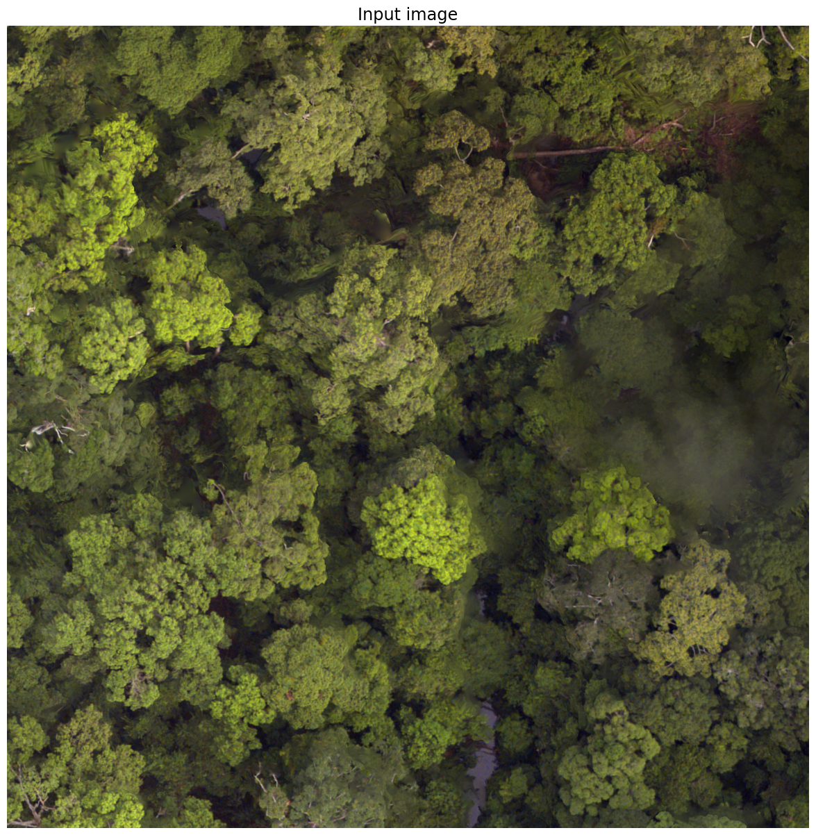
Read in and display the PNG file#
Show code cell source
im = cv2.imread(filepath)
plot_input = plt.figure(figsize=(15,15))
plt.imshow(Image.fromarray(im))
plt.title('Input image',fontsize='xx-large')
plt.axis('off')
plt.show()
Modelling#
Download the pretrained model#
# define the URL to retrieve the model
fn = 'model_final.pth'
url = f'https://zenodo.org/record/5515408/files/{fn}?download=1'

urllib.request.urlretrieve(url, config['model'] + '/' + fn)
('./notebook/model/model_final.pth',
 <http.client.HTTPMessage at 0x7fc1e9303400>)
Settings of detectron2 config#
The following lines allow configuring the main settings for predictions and load them into a DefaultPredictor object.
cfg = get_cfg()

# if you want to make predictions using a CPU, run the following line. If using GPU, hash it out.
cfg.MODEL.DEVICE='cpu'

# model and hyperparameter selection
cfg.merge_from_file(model_zoo.get_config_file("COCO-InstanceSegmentation/mask_rcnn_R_101_FPN_3x.yaml"))
cfg.DATALOADER.NUM_WORKERS = 2
cfg.SOLVER.IMS_PER_BATCH = 2
cfg.MODEL.ROI_HEADS.NUM_CLASSES = 1

### path to the saved pre-trained model weights
cfg.MODEL.WEIGHTS = config['model'] + '/model_final.pth'

# set confidence threshold at which we predict
cfg.MODEL.ROI_HEADS.SCORE_THRESH_TEST = 0.15

#### Settings for predictions using detectron config

predictor = DefaultPredictor(cfg)
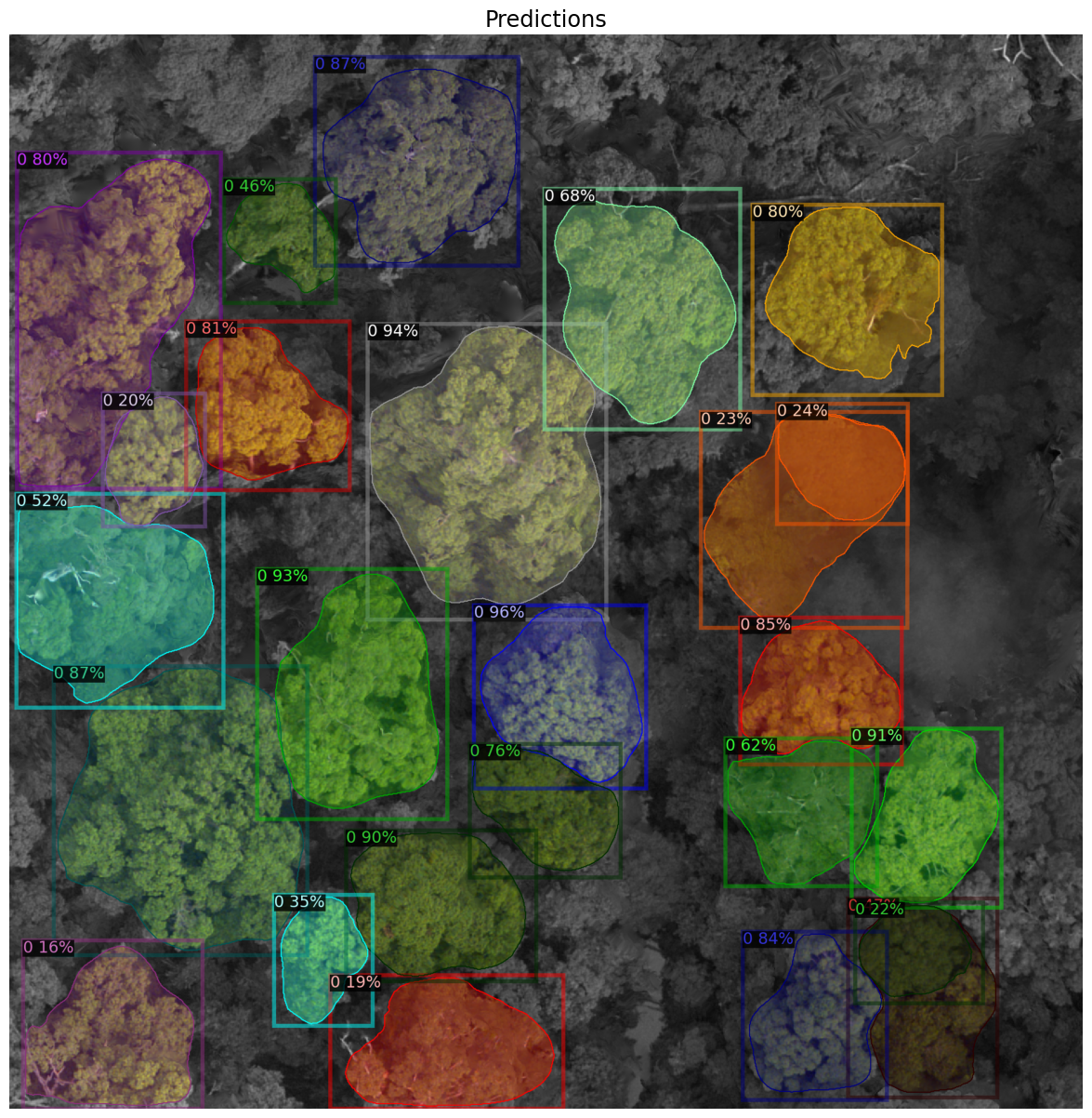
Outputs#
Showing the predictions from detectreeRGB#
Show code cell source
outputs = predictor(im)
v = Visualizer(im[:, :, ::-1], scale=1.5, instance_mode=ColorMode.IMAGE_BW)   # remove the colors of unsegmented pixels
v = v.draw_instance_predictions(outputs["instances"].to("cpu"))
image = cv2.cvtColor(v.get_image()[:, :, :], cv2.COLOR_BGR2RGB)

plot_predictions = plt.figure(figsize=(15,15))
plt.imshow(Image.fromarray(image))
plt.title('Predictions',fontsize='xx-large')
plt.axis('off')
plt.show()
Convert predictions into geospatial files#
To GeoTIFF#
mask_array = outputs['instances'].pred_masks.cpu().numpy()

# get confidence scores too
mask_array_scores = outputs['instances'].scores.cpu().numpy()

num_instances = mask_array.shape[0]
mask_array_instance = []
output = np.zeros_like(mask_array)

mask_array_instance.append(mask_array)
output = np.where(mask_array_instance[0] == True, 255, output)
fresh_output = output.astype(float)
x_scaling = 140/fresh_output.shape[1]
y_scaling = 140/fresh_output.shape[2]
# this is an affine transform. This needs to be altered significantly.
transform = from_origin(int(filepath[-17:-11])-20, int(filepath[-10:-4])+120, y_scaling, x_scaling)

output_raster = config['out_geotiff'] + '/' + 'predicted_rasters_' + filepath[-17:-4]+ '.tif'

new_dataset = rasterio.open(output_raster, 'w', driver='GTiff',
                                height = fresh_output.shape[1], width = fresh_output.shape[2], count = fresh_output.shape[0],
                                dtype=str(fresh_output.dtype),
                                crs='+proj=utm +zone=50 +datum=WGS84 +units=m +no_defs',
                                transform=transform)

new_dataset.write(fresh_output)
new_dataset.close()
To shapefile#
# Read input band with Rasterio

with rasterio.open(output_raster) as src:
    shp_schema = {'geometry': 'MultiPolygon','properties': {'pixelvalue': 'int', 'score': 'float'}}

    crs = src.crs
    for i in range(src.count):
        src_band = src.read(i+1)
        src_band = np.float32(src_band)
        conf = mask_array_scores[i]
        # Keep track of unique pixel values in the input band
        unique_values = np.unique(src_band)
        # Polygonize with Rasterio. `shapes()` returns an iterable
        # of (geom, value) as tuples
        shapes = list(rasterio.features.shapes(src_band, transform=src.transform))

        if i == 0:
            with fiona.open(config['out_shapefile'] + '/predicted_polygons_' + filepath[-17:-4] + '_' + str(0) + '.shp', 'w', 'ESRI Shapefile',
                            shp_schema) as shp:
                polygons = [shape(geom) for geom, value in shapes if value == 255.0]
                multipolygon = MultiPolygon(polygons)
                        # simplify not needed here
                        #multipolygon = multipolygon_a.simplify(0.1, preserve_topology=False)
                shp.write({
                          'geometry': mapping(multipolygon),
                          'properties': {'pixelvalue': int(unique_values[1]), 'score': float(conf)}
                           })
        else:
            with fiona.open(config['out_shapefile'] + '/predicted_polygons_' + filepath[-17:-4] + '_' + str(0)+'.shp', 'a', 'ESRI Shapefile',
                            shp_schema) as shp:
                polygons = [shape(geom) for geom, value in shapes if value == 255.0]
                multipolygon = MultiPolygon(polygons)
                        # simplify not needed here
                        #multipolygon = multipolygon_a.simplify(0.1, preserve_topology=False)
                shp.write({
                          'geometry': mapping(multipolygon),
                          'properties': {'pixelvalue': int(unique_values[1]), 'score': float(conf)}
                           })
Interactive map to visualise the exported files#
Plot tree crown delineation predictions and scores#
Show code cell source
# load and plot polygons
in_shp = glob.glob(config['out_shapefile'] + '/*.shp')

poly_df = gpd.read_file(in_shp[0])

plot_vector = poly_df.hvplot(hover_cols=['score'], legend=False).opts(fill_color=None,line_color=None,alpha=0.5, width=800, height=600, xaxis=None, yaxis=None)
plot_vector
Plot the exported GeoTIFF file#
Show code cell source
# load and plot RGB image
r = tc_rgb.sel(band=[1,2,3])

normalized = r/(r.quantile(.99,skipna=True)/255)

mask = normalized.where(normalized < 255)

int_arr = mask.astype(int)

plot_rgb = int_arr.astype('uint8').hvplot.rgb(
    x='x', y='y', bands='band', data_aspect=0.8, hover=False, legend=False, rasterize=True, xaxis=None, yaxis=None, title='Tree crown delineation by detectreeRGB'
)
Overlay the prediction labels and image#
Note we have some artifacts in the RGB image due to the transformations using the normalization procedure.
Show code cell source
plot_predictions_interactive = plot_rgb * plot_vector
plot_predictions_interactive
OMP: Info #276: omp_set_nested routine deprecated, please use omp_set_max_active_levels instead.
Save plot#
hvplot.save(plot_predictions_interactive, notebook_folder + '/interactive_predictions.html')
Summary#
We have read in a raster, chosen a tile and made predictions on it. These predictions can then be transformed to shapefiles and examined in GIS software!
We made the predictions on the
pngusing a pretrained Mask R-CNN model,detectreeRGB.The outputs showed the model capability to detect and delineate tree crowns from aerial imagery.
We then extracted our predictions, added the geospatial location back in, and exported them as shapefiles including the confidence score assigned to each prediction by the model.
Visualised the predictions on an interactive map!
Citing this Notebook#
Please see CITATION.cff for the full citation information. The citation file can be exported to APA or BibTex formats (learn more here).
Additional information#
Codebase: version 1.0.0 with commit 16a5a1c
License: The code in this notebook is licensed under the MIT License. The Environmental Data Science book is licensed under the Creative Commons by Attribution 4.0 license. See further details here.
Contact: If you have any suggestion or report an issue with this notebook, feel free to create an issue or send a direct message to environmental.ds.book@gmail.com.
Notebook repository version: v1.0.4
Last tested: 2024-03-12