Tree crown detection using DeepForest

Forest Modelling Standard Python

Context

Purpose

Detect tree crown using a state-of-art Deep Learning model for object detection.

Modelling approach

A prebuilt Deep Learning model, named DeepForest, is used to predict individual tree crowns from an airborne RGB image. DeepForest was trained on data from the National Ecological Observatory Network (NEON). DeepForest was implemented in Python 3.7 using initally Tensorflow v1.14 but later moved to Pytorch. Further details can be found in the package documentation.

Highlights

• Fetch a NEON sample image from a Zenodo repository.

• Retrieve and plot the reference annotations (bounding boxes) for the target image.

• Load and use a pretrained DeepForest model to generate full-image or tile-wise prediction.

• Indicate the pros and cons of full-image and tile-wise prediction.

Contributions

Notebook

• Alejandro Coca-Castro (author), The Alan Turing Institute, @acocac

• Matt Allen (reviewer), Department of Geography - University of Cambridge, @mja2106

Modelling codebase

• Ben Weinstein (maintainer & developer), University of Florida, @bw4sz

• Henry Senyondo (support maintainer), University of Florida, @henrykironde

• Ethan White (PI and author), University of Florida, @weecology

• Other contributors are listed in the GitHub repo

Modelling publications

• Ben G Weinstein, Sergio Marconi, Mélaine Aubry-Kientz, Gregoire Vincent, Henry Senyondo, and Ethan P White. Deepforest: a python package for rgb deep learning tree crown delineation. Methods in Ecology and Evolution, 11:1743–1751, 2020. URL: https://besjournals.onlinelibrary.wiley.com/doi/abs/10.1111/2041-210X.13472, doi:https://doi.org/10.1111/2041-210X.13472.

• Ben G Weinstein, Sergio Marconi, Stephanie Bohlman, Alina Zare, and Ethan White. Individual tree-crown detection in rgb imagery using semi-supervised deep learning neural networks. Remote Sensing, 2019. URL: https://www.mdpi.com/2072-4292/11/11/1309, doi:10.3390/rs11111309.

• Ben G Weinstein, Sergio Marconi, Stephanie A Bohlman, Alina Zare, and Ethan P White. Cross-site learning in deep learning rgb tree crown detection. Ecological Informatics, 56:101061, 2020. URL: https://www.sciencedirect.com/science/article/pii/S157495412030011X, doi:https://doi.org/10.1016/j.ecoinf.2020.101061.

Note

The author acknowledges DeepForest contributors. Some code snippets were extracted from DeepForest GitHub public repository.

Install and load libraries

Show code cell source Hide code cell source

!pip -q install torchvision==0.10.0
!pip -q install torch==1.9.0
!pip -q install DeepForest==1.0.0
!pip -q install geoviews

WARNING: The directory '/home/jovyan/.cache/pip' or its parent directory is not owned or is not writable by the current user. The cache has been disabled. Check the permissions and owner of that directory. If executing pip with sudo, you should use sudo's -H flag.
WARNING: Running pip as the 'root' user can result in broken permissions and conflicting behaviour with the system package manager. It is recommended to use a virtual environment instead: https://pip.pypa.io/warnings/venv
WARNING: The directory '/home/jovyan/.cache/pip' or its parent directory is not owned or is not writable by the current user. The cache has been disabled. Check the permissions and owner of that directory. If executing pip with sudo, you should use sudo's -H flag.
WARNING: Running pip as the 'root' user can result in broken permissions and conflicting behaviour with the system package manager. It is recommended to use a virtual environment instead: https://pip.pypa.io/warnings/venv
WARNING: The directory '/home/jovyan/.cache/pip' or its parent directory is not owned or is not writable by the current user. The cache has been disabled. Check the permissions and owner of that directory. If executing pip with sudo, you should use sudo's -H flag.
WARNING: Running pip as the 'root' user can result in broken permissions and conflicting behaviour with the system package manager. It is recommended to use a virtual environment instead: https://pip.pypa.io/warnings/venv
WARNING: The directory '/home/jovyan/.cache/pip' or its parent directory is not owned or is not writable by the current user. The cache has been disabled. Check the permissions and owner of that directory. If executing pip with sudo, you should use sudo's -H flag.
WARNING: Running pip as the 'root' user can result in broken permissions and conflicting behaviour with the system package manager. It is recommended to use a virtual environment instead: https://pip.pypa.io/warnings/venv

Show code cell source Hide code cell source

import glob
import os
import urllib
import numpy as np

import intake
import matplotlib.pyplot as plt
import xmltodict
import cv2

import torch

from shapely.geometry import box
import pandas as pd
from geopandas import GeoDataFrame
import xarray as xr
import panel as pn
import holoviews as hv
import hvplot.pandas
import hvplot.xarray
from skimage.exposure import equalize_hist

import pooch

import warnings
warnings.filterwarnings(action='ignore')

hv.extension('bokeh', width=100)
%matplotlib inline

Set project structure

notebook_folder = './notebook'
if not os.path.exists(notebook_folder):
    os.makedirs(notebook_folder)

Fetch a RGB image from Zenodo

Fetch a sample image from a publicly accessible location.

pooch.retrieve(
    url="doi:10.5281/zenodo.3459803/2018_MLBS_3_541000_4140000_image_crop.tif",
    known_hash="md5:01a7cf23b368ff9e006fda8fe9ca4c8c",
    path=notebook_folder,
    fname="2018_MLBS_3_541000_4140000_image_crop.tif"
)

Downloading data from 'doi:10.5281/zenodo.3459803/2018_MLBS_3_541000_4140000_image_crop.tif' to file '/home/jovyan/notebook/2018_MLBS_3_541000_4140000_image_crop.tif'.

'/home/jovyan/notebook/2018_MLBS_3_541000_4140000_image_crop.tif'

# set catalogue location
catalog_file = os.path.join(notebook_folder, 'catalog.yaml')

with open(catalog_file, 'w') as f:
    f.write('''
sources:
  NEONTREE_rgb:
    driver: xarray_image
    description: 'NeonTreeEvaluation RGB images (collection)'
    args:
      urlpath: "{{ CATALOG_DIR }}/2018_MLBS_3_541000_4140000_image_crop.tif"
      ''')

Load an intake catalog for the downloaded data.

cat_tc = intake.open_catalog(catalog_file)

Load sample image

Here we use intake to load the image through dask.

tc_rgb = cat_tc["NEONTREE_rgb"].to_dask()
tc_rgb

<xarray.DataArray (y: 1864, x: 1429, channel: 3)> Size: 8MB
dask.array<xarray-<this-array>, shape=(1864, 1429, 3), dtype=uint8, chunksize=(1864, 1429, 3), chunktype=numpy.ndarray>
Coordinates:
  * y        (y) int64 15kB 0 1 2 3 4 5 6 ... 1857 1858 1859 1860 1861 1862 1863
  * x        (x) int64 11kB 0 1 2 3 4 5 6 ... 1422 1423 1424 1425 1426 1427 1428
  * channel  (channel) int64 24B 0 1 2

xarray.DataArray

• y: 1864
• x: 1429
• channel: 3

• dask.array<chunksize=(1864, 1429, 3), meta=np.ndarray>

  Array Chunk Bytes 7.62 MiB 7.62 MiB Shape (1864, 1429, 3) (1864, 1429, 3) Dask graph 1 chunks in 1 graph layer Data type uint8 numpy.ndarray

• Coordinates: (3)
  • y
    (y)
    int64
    0 1 2 3 4 ... 1860 1861 1862 1863

    array([   0,    1,    2, ..., 1861, 1862, 1863])

  • x
    (x)
    int64
    0 1 2 3 4 ... 1425 1426 1427 1428

    array([   0,    1,    2, ..., 1426, 1427, 1428])

  • channel
    (channel)
    int64
    0 1 2

    array([0, 1, 2])

• Indexes: (3)
  • y
    PandasIndex

    PandasIndex(Index([   0,    1,    2,    3,    4,    5,    6,    7,    8,    9,
           ...
           1854, 1855, 1856, 1857, 1858, 1859, 1860, 1861, 1862, 1863],
          dtype='int64', name='y', length=1864))

  • x
    PandasIndex

    PandasIndex(Index([   0,    1,    2,    3,    4,    5,    6,    7,    8,    9,
           ...
           1419, 1420, 1421, 1422, 1423, 1424, 1425, 1426, 1427, 1428],
          dtype='int64', name='x', length=1429))

  • channel
    PandasIndex

    PandasIndex(Index([0, 1, 2], dtype='int64', name='channel'))

• Attributes: (0)

Load and prepare labels

# functions to load xml and extract bounding boxes

# function to create ordered dictionary of .xml annotation files
def loadxml(imagename):
    imagename = imagename.replace('.tif','')
    fullurl = "https://raw.githubusercontent.com/weecology/NeonTreeEvaluation/master/annotations/" + imagename + ".xml"
    file = urllib.request.urlopen(fullurl)
    data = file.read()
    file.close()
    data = xmltodict.parse(data)
    return data

# function to extract bounding boxes
def extractbb(i):
    bb = [f['bndbox'] for f in allxml[i]['annotation']['object']]
    return bb

filenames = glob.glob(os.path.join(notebook_folder, '*.tif'))
filesn = [os.path.basename(i) for i in filenames]

allxml = [loadxml(i) for i in filesn]
bball = [extractbb(i) for i in range(0,len(allxml))]
print(len(bball))

1

Visualise image and labels

# function to plot images
def cv2_imshow(a, **kwargs):
    a = a.clip(0, 255).astype('uint8')
    # cv2 stores colors as BGR; convert to RGB
    if a.ndim == 3:
        if a.shape[2] == 4:
            a = cv2.cvtColor(a, cv2.COLOR_BGRA2RGBA)
        else:
            a = cv2.cvtColor(a, cv2.COLOR_BGR2RGB)

    return plt.imshow(a, **kwargs)

image = tc_rgb

# plot predicted bbox
image2 = image.values.copy()
target_bbox = bball[0]
print(type(target_bbox))
print(target_bbox[0:2])

<class 'list'>
[{'xmin': '1377', 'ymin': '697', 'xmax': '1429', 'ymax': '752'}, {'xmin': '787', 'ymin': '232', 'xmax': '811', 'ymax': '256'}]

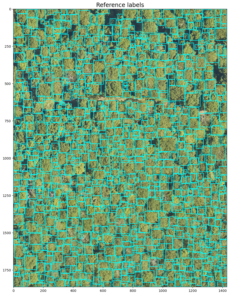
Show code cell source Hide code cell source

for row in target_bbox:
    cv2.rectangle(image2, (int(row["xmin"]), int(row["ymin"])), (int(row["xmax"]), int(row["ymax"])), (0,255,255), thickness=2, lineType=cv2.LINE_AA)

plot_reference = plt.figure(figsize=(15,15))
cv2_imshow(np.flip(image2,2))
plt.title('Reference labels',fontsize='xx-large')
plt.show()

Load DeepForest pretrained model

Now we’re going to load and use a pretrained model from the deepforest package.

from deepforest import main

# load deep forest model
model = main.deepforest()
model.use_release()
model.current_device = torch.device("cpu")

Reading config file: /srv/conda/envs/notebook/lib/python3.9/site-packages/deepforest/data/deepforest_config.yml

Downloading: "https://download.pytorch.org/models/retinanet_resnet50_fpn_coco-eeacb38b.pth" to /home/jovyan/.cache/torch/hub/checkpoints/retinanet_resnet50_fpn_coco-eeacb38b.pth
100%|██████████| 130M/130M [00:00<00:00, 266MB/s]

Downloading model from DeepForest release 1.0.0, see https://github.com/weecology/DeepForest/releases/tag/1.0.0 for details

NEON.pt: 129MB [00:00, 241MB/s]                            

Model was downloaded and saved to /srv/conda/envs/notebook/lib/python3.9/site-packages/deepforest/data/NEON.pt
Loading pre-built model: https://github.com/weecology/DeepForest/releases/tag/1.0.0

pred_boxes = model.predict_image(image=image.values)
print(pred_boxes.head(5))

     xmin   ymin    xmax   ymax label     score
0  1258.0  561.0  1399.0  698.0  Tree  0.415253
1  1119.0  527.0  1255.0  660.0  Tree  0.395936
2     7.0  248.0   140.0  395.0  Tree  0.376462
3   444.0  459.0   575.0  582.0  Tree  0.355282
4    94.0  149.0   208.0  260.0  Tree  0.347174

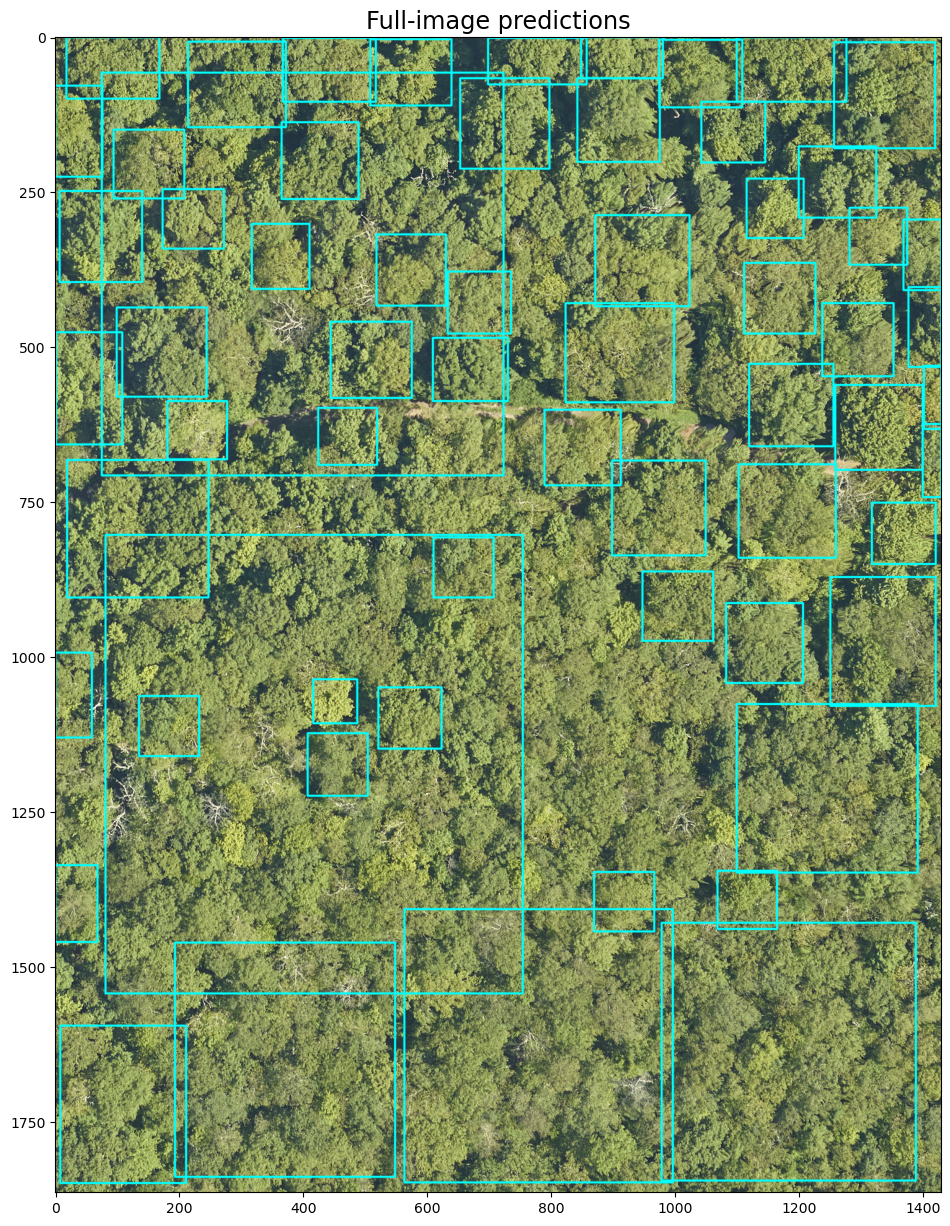
Show code cell source Hide code cell source

image3 = image.values.copy() 

for index, row in pred_boxes.iterrows():
    cv2.rectangle(image3, (int(row["xmin"]), int(row["ymin"])), (int(row["xmax"]), int(row["ymax"])), (0,255,255), thickness=2, lineType=cv2.LINE_AA)

plot_fullimage = plt.figure(figsize=(15,15))
cv2_imshow(np.flip(image3,2))
plt.title('Full-image predictions',fontsize='xx-large')
plt.show()

Comparison full image prediction and reference labels

Let’s compare the labels and predictions over the tested image.

Show code cell source Hide code cell source

plot_referandfullimage = plt.figure(figsize=(15,15))
ax1 = plt.subplot(1, 2, 1), cv2_imshow(np.flip(image2,2))
ax1[0].set_title('Reference labels',fontsize='xx-large')
ax2 = plt.subplot(1, 2, 2), cv2_imshow(np.flip(image3,2))
ax2[0].set_title('Full-image predictions', fontsize='xx-large')
plt.show() # To show figure

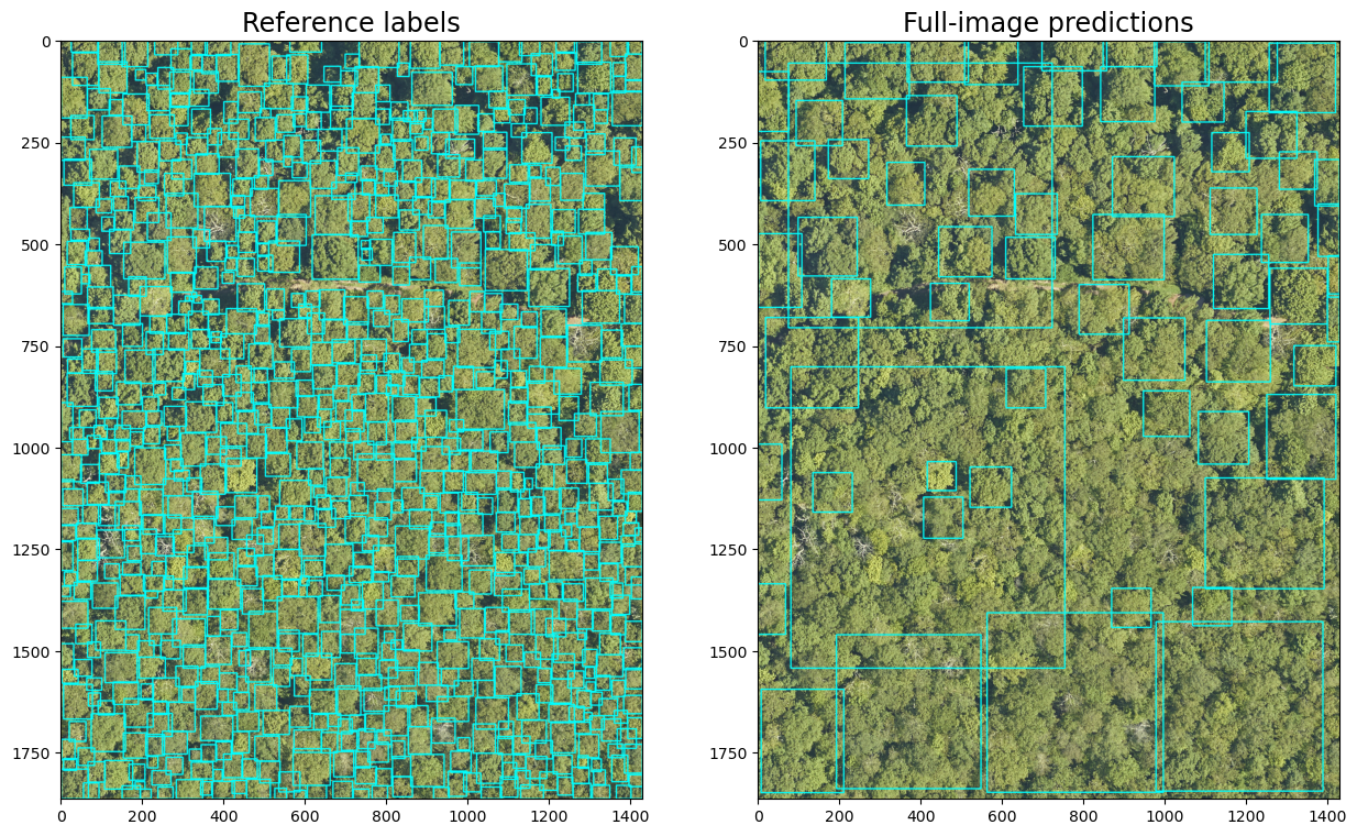
Interpretation:

• It seems the pretrained model doesn’t perform well with the tested image.

• The low performance might be explained due to the pretrained model used 10 cm resolution images.

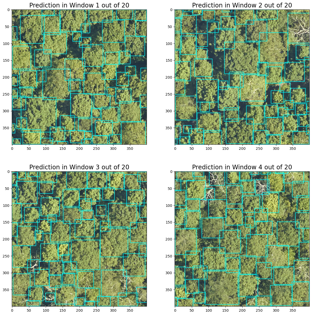
Tile-based prediction

To optimise the predictions, the DeepForest can be run tile-wise.

The following cells show how to define the optimal window i.e. tile size.

from deepforest import preprocess

#Create windows of 400px
windows = preprocess.compute_windows(image.values, patch_size=400,patch_overlap=0)
print(f'We have {len(windows)} windows in the image')

We have 20 windows in the image

Show code cell source Hide code cell source

#Loop through a few sample windows, crop and predict
plot_tilewindows, axes, = plt.subplots(nrows=2,ncols=2, figsize=(15,15))
axes = axes.flatten()
for index2 in range(4):
    crop = image.values[windows[index2].indices()]
    #predict in bgr channel order, color predictions in red.
    boxes = model.predict_image(image=np.flip(crop[...,::-1],2), return_plot = True)

    #but plot in rgb channel order
    axes[index2].imshow(boxes[...,::-1])
    axes[index2].set_title(f'Prediction in Window {index2 + 1} out of {len(windows)}', fontsize='xx-large')

Once a suitable tile size is defined, we can run in a batch using the predict_tile function:

Show code cell source Hide code cell source

tile = model.predict_tile(image=image.values,return_plot=False,patch_overlap=0,iou_threshold=0.05,patch_size=400)

# plot predicted bbox
image_tile = image.values.copy()

for index, row in tile.iterrows():
    cv2.rectangle(image_tile, (int(row["xmin"]), int(row["ymin"])), (int(row["xmax"]), int(row["ymax"])), (0, 255, 255), thickness=2, lineType=cv2.LINE_AA)

plot_tilewise = plt.figure(figsize=(15,15))
ax1 = plt.subplot(1, 2, 1), cv2_imshow(np.flip(image2,2))
ax1[0].set_title('Reference labels',fontsize='xx-large')
ax2 = plt.subplot(1, 2, 2), cv2_imshow(np.flip(image_tile,2))
ax2[0].set_title('Tile-wise predictions', fontsize='xx-large')
plt.show() # To show figure

100%|██████████| 20/20 [00:33<00:00,  1.65s/it]

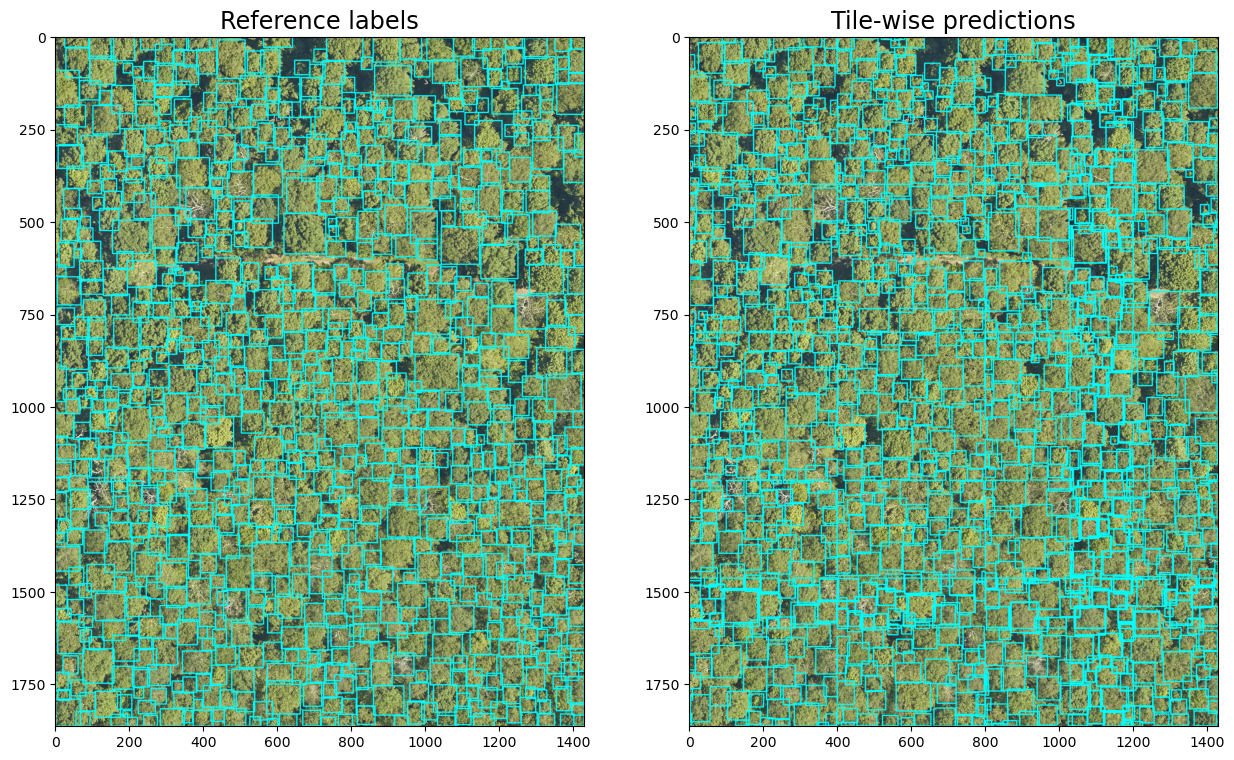
Interpretation

• The tile-based prediction provides more reasonable results than predicting over the whole image.

• While the prediction looks closer to the reference labels, there seem to be some tiles edges artefacts. This will require further investigation i.e. inspecting the deepforest tile-wise prediction function to understand how predictions from different tiles are combined after the model has made them.

Interactive plots

The plot below summarises above static plots by interactively comparing bounding boxes and scores of full-image and tile-wise predictions. To zoom-in the reference NEON RGB image with its original resolution change rasterize=True to rasterize=False.

Show code cell source Hide code cell source

## function to convert bbox in dictionary to geopandas
def bbox_to_geopandas(bbox_df):
    geometry = [box(x1, y1, x2, y2) for x1,y1,x2,y2 in zip(bbox_df.xmin, bbox_df.ymin, bbox_df.xmax, bbox_df.ymax)]
    poly_geo = GeoDataFrame(bbox_df, geometry=geometry)
    return poly_geo

## prepare reference and prediction bbox
### convert data types for reference bbox dictionary
reference = pd.DataFrame.from_dict(target_bbox)
reference[['xmin', 'ymin', 'xmax', 'ymax']] = reference[['xmin', 'ymin', 'xmax', 'ymax']].astype(int)

poly_reference = bbox_to_geopandas(reference)
poly_prediction_image = bbox_to_geopandas(pred_boxes)
poly_prediction_tile = bbox_to_geopandas(tile)

## settings for hvplot objects
settings_vector = dict(fill_color=None, width=400, height=400, clim=(0,1), fontsize={'title': '110%'})
settings_image = dict(x='x', y='y', data_aspect=1, xaxis=False, yaxis=None)

## create hvplot objects
plot_RGB = tc_rgb.hvplot.rgb(**settings_image, bands='channel', hover=False, rasterize=True)
plot_vector_reference = poly_reference.hvplot(hover_cols=False, legend=False).opts(title='Reference labels', alpha=1, **settings_vector)
plot_vector_image = poly_prediction_image.hvplot(hover_cols=['score'], legend=False).opts(title='Full-image predictions', alpha=0.5, **settings_vector)
plot_vector_tile = poly_prediction_tile.hvplot(hover_cols=['score'], legend=False).opts(title='Tile-wise predictions', alpha=0.5, **settings_vector)

plot_comparison = pn.Row(pn.Column(plot_RGB * plot_vector_reference, 
                         plot_RGB * plot_vector_image),
                         pn.Column(pn.Spacer(background='white', width=400, height=400),  
                         plot_RGB * plot_vector_tile), scroll=True)

plot_comparison.embed()

Summary

This notebook has demonstrated the use of:

• pooch and intake package to fetch data from a Zenodo repository containing training data files of the NeonTreeEvaluation Benchmark.

• deepforest package to easily load and run a pretrained model for tree crown classification from very-high resolution RGB imagery.

• The tile-wise option in deepforest considerably improve tree crown predictions. However, the user should define an optimal tile size.

• cv2 to generate static plots comparing reference against bounding boxes and scores of two prediction strategies, full-image and tile-wise predictions.

• hvplot and panel to interactively compare both prediction strategies against reference labels.

Citing this Notebook

Please see CITATION.cff for the full citation information. The citation file can be exported to APA or BibTex formats (learn more here).

Additional information

License: The code in this notebook is licensed under the MIT License. The Environmental Data Science book is licensed under the Creative Commons by Attribution 4.0 license. See further details here.

Contact: If you have any suggestion or report an issue with this notebook, feel free to create an issue or send a direct message to environmental.ds.book@gmail.com.

from datetime import date

print('Notebook repository version: v1.0.4')
print(f'Last tested: {date.today()}')

Notebook repository version: v1.0.4
Last tested: 2024-03-11